How to Get Historical Exchange Rates in Google Sheets

Sometimes today's exchange rate is the wrong one. You might be closing out last month's books and need the rate from the last day of the period, or you're filing an expense report for a trip you took six weeks ago, or you need to verify what a payment was actually worth when it cleared. In all of those cases, you need a historical rate rather than whatever the market is doing right now. This guide covers how to pull those past rates directly into Google Sheets using GOOGLEFINANCE.

Getting a rate for a specific date

Here's the formula for a single historical rate:

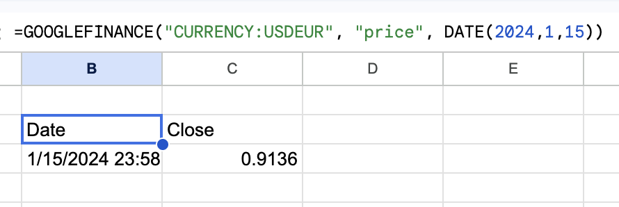
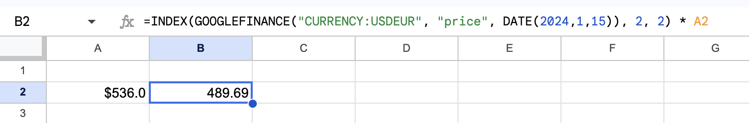
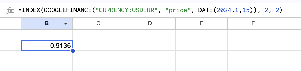
=INDEX(GOOGLEFINANCE("CURRENCY:USDEUR", "price", DATE(2024,1,15)), 2, 2)

The INDEX wrapper might look unnecessary, but it's actually required. When you pass a date to GOOGLEFINANCE, it doesn't give you back a single number. It returns a small two-column table: a header row with the labels "Date" and "Close", followed by a data row with the actual values. If you try to use that table directly (say, multiply it by a dollar amount), Google Sheets throws an error because it doesn't know how to multiply a table by a number.

INDEX(_, 2, 2) solves this by extracting one specific cell from that table. The 2, 2 means row 2, column 2, which is where the actual rate sits.

Once you have that, multiplying it by a cell value works the same way as with a live rate:

=INDEX(GOOGLEFINANCE("CURRENCY:USDEUR", "price", DATE(2024,1,15)), 2, 2) * A2

This takes whatever dollar amount is in A2 and converts it to euros at the January 15, 2024 rate.

Note that the formula above uses the DATE() function rather than a text string like "2024-01-15". Either will work in many cases, but DATE() is more reliable. If your spreadsheet is shared with people in different locales, or if you're using a template, date strings can be parsed differently depending on regional settings. DATE() doesn't have that ambiguity.

Getting rates for a range of dates

If you need rates across multiple days (for example, to track how a currency moved over a month) you can pass a start and end date:

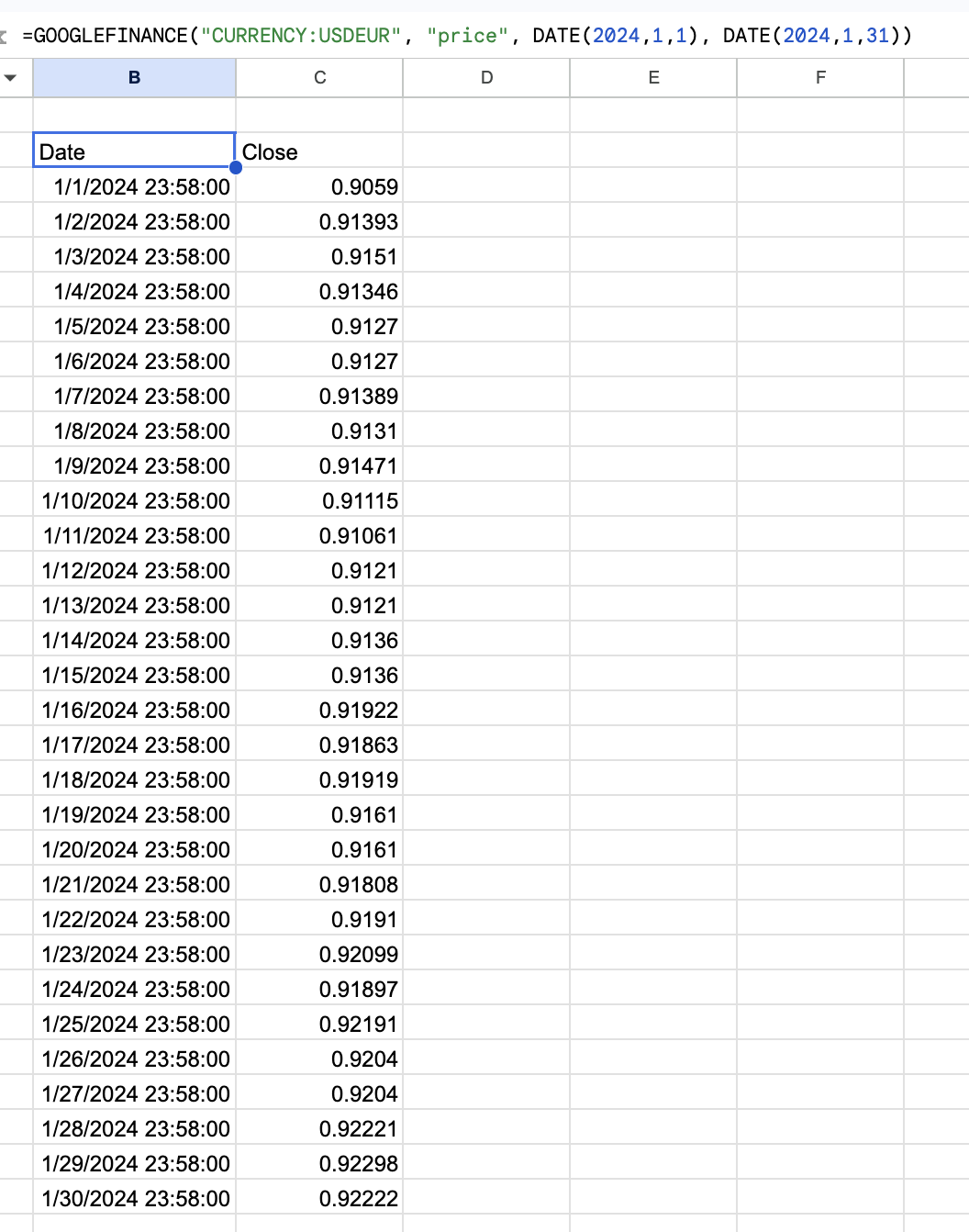
=GOOGLEFINANCE("CURRENCY:USDEUR", "price", DATE(2024,1,1), DATE(2024,1,31))

This spills automatically into multiple rows. The first row is a header, and every row after that is one day with its date and closing rate. No INDEX needed here. You want the full table, not a single value.

This is useful for building a chart. Paste the formula in a cell, let it expand, then insert a chart using that range. You can see at a glance how the rate moved across a period.

One thing to keep in mind: the output from this formula occupies as many rows as there are trading days in the range. If other data sits below where you put the formula, it will get overwritten. Put the formula somewhere with clear space below it, or dedicate a separate sheet to the output.

Formatting the output

Two formatting issues come up almost every time.

First, the date column often shows serial numbers instead of readable dates. In Google Sheets, dates are stored internally as numbers (the number of days since December 30, 1899), and the GOOGLEFINANCE output sometimes comes through without the date format applied. To fix it, select the column, go to Format > Number > Date, and it'll display correctly.

Second, the rate column is just a raw decimal. Format it however your spreadsheet needs. You might want four decimal places for precision, or two if you're using it in a presentation. Go to Format > Number > Custom number format and enter something like 0.0000 for four decimal places.

Things to know

Date format issues. As mentioned above, use DATE() instead of text strings to stay out of trouble with locale-dependent date parsing. DATE(2024, 1, 15) means January 15, 2024 in every locale. "1/15/2024" does not.

Mid-market rates. GOOGLEFINANCE uses mid-market rates, which sit in the middle between the buy and sell rates. Your bank uses a rate with a spread added on top, which is how they make money on currency exchanges. The numbers you see in Sheets will be slightly different from what appeared on your bank statement or payment processor receipt. For accounting purposes, you may need to check your bank's historical rate rather than rely on GOOGLEFINANCE.

Currency pairs that aren't available. Not every currency pair is in Google Finance. Major pairs (USD/EUR, GBP/USD, USD/JPY) work reliably. Some less-common currencies return #N/A. If you're getting that error and your currency code looks correct, try checking whether the pair exists at all in Google Finance before assuming the formula is wrong.

What if you need the rate for a cell reference date?

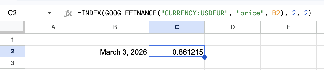
You can replace the DATE() arguments with cell references. If the date you want is in cell B2:

=INDEX(GOOGLEFINANCE("CURRENCY:USDEUR", "price", B2), 2, 2)

Make sure B2 is formatted as a date in Google Sheets, not as text. If you typed the date as plain text, GOOGLEFINANCE may not recognize it. You can verify the format by selecting the cell and checking Format > Number. It should say "Date", not "Plain text" or "Automatic".

This approach works well if you have a column of transaction dates and want to look up each one automatically. Put the GOOGLEFINANCE formula in the column next to the dates, with B2 (or whatever the first date cell is) as the date argument, then drag it down.

Building a conversion table with dynamic dates

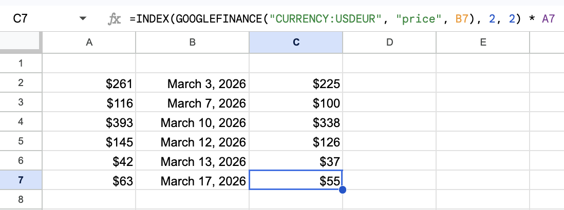
Here's a setup that comes up often in expense reporting: a column of amounts in column A, a column of dates in column B, and you need the converted value for each row based on that row's date.

In column C:

=INDEX(GOOGLEFINANCE("CURRENCY:USDEUR", "price", B2), 2, 2) * A2

Drag that down through all your rows. Each row picks up the rate for its own date. The result is a column of converted values where each one used the correct historical rate.

One caveat: each GOOGLEFINANCE call counts as a separate data request. In a spreadsheet with hundreds of rows, this can slow things down or occasionally hit rate limits. For large datasets, it may be more practical to look up unique dates separately, pull the rates into a reference table, and use VLOOKUP or XLOOKUP to match them. That way each unique date is only queried once.

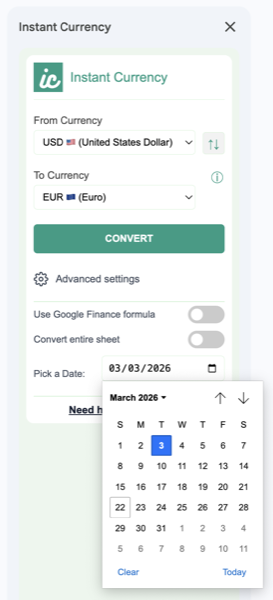
Instant Currency

If you'd rather not deal with the INDEX wrapping, Instant Currency has a date picker for historical lookups. You pick the currencies, pick the date, and it handles the formula construction and formatting automatically. It also converts cells directly, which is useful when you don't need the formulas at all and just want the numbers.

For general currency conversion formulas, see our step-by-step GOOGLEFINANCE guide. If you have questions about a specific use case, get in touch. We're happy to help.