Google Sheets Currency Conversion with Live Exchange Rates

If you deal with different currencies in Google Sheets, you know that it can be a pain to look up exchange rates, paste them into your spreadsheet, then calculate the converted value. Luckily, there's a formula that makes this much easier. The GOOGLEFINANCE formula, beyond providing real-time information about stocks, can also give you exchange rates for dozens of currencies.

By the end of this tutorial, you'll know how to use the GOOGLEFINANCE formula for live currency conversion and format cells with proper currency symbols.

What is GOOGLEFINANCE?

GOOGLEFINANCE is a formula built into Google Sheets that offers current and past information from Google Finance directly in your spreadsheet. You can look up market information, prices on specific stocks, and historical or current currency rates. It's all free within Google Sheets and requires just a few steps to set up.

Can I use GOOGLEFINANCE in Excel?

No, GOOGLEFINANCE is limited to Google Sheets. Excel has its own currency and market look-up tools, and two systems won't work together. If you download a Google Sheets spreadsheet with a GOOGLEFINANCE formula as XLSX, that formula will break when you open it in Excel. Similarly, if you upload an XLSX with Excel's currency tools into Google Sheets, it will either break entirely or simply hard code the values, losing the live connection.

How to convert currencies with GOOGLEFINANCE: A step-by-step guide

In this example, we'll assume that you're already using Google Sheets and have currency amounts that you want to convert. If you want to try this out with a test spreadsheet, just go to sheets.new to create a dummy spreadsheet. That creates a spreadsheet in whichever Google account you're currently logged into.

We'll be using the example of converting British Pounds to US dollars, but we'll also show you how to convert other currencies.

Step 1: Decide where you want the converted currency

In this example, imagine that we need to make an expense report for a trip to London. We've got a list of amounts in pounds in column B.

The thing you need to know about the GOOGLEFINANCE formula is that it won't replace the pound amount with the converted value in dollars. Like any other Sheets formula, you have your inputs in one place, then you'll put the formula where you want the output.

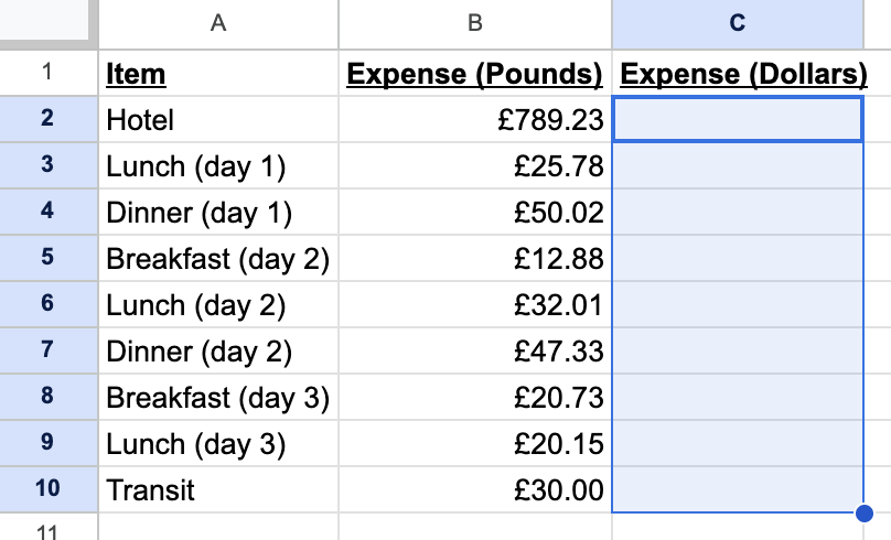
In this case, it makes sense to have the dollar amounts right next to their equivalent pound values, so we'll put the formulas in column C.

Step 2: Build the formula

The basic structure of a GOOGLEFINANCE currency formula is this:

=GOOGLEFINANCE("CURRENCY:[original currency][target currency]")

There's no space space anywhere in the formula. In our example, to get the exchange from pounds to dollars, we'd use this:

=GOOGLEFINANCE("CURRENCY:GBPUSD")

Notice a few things:

• The formula uses three-letter codes for currencies, not their names. Wikipedia has a helpful list of all currencies that use these codes.
• Everything is squished together. In the middle of the formula you have GBPUSD.

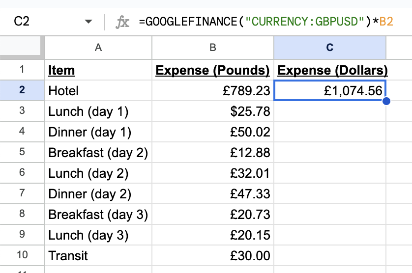
This formula gives you the exchange rate. If that's all you want, great. But if you want to convert specific values, the way we have in our example, you'll need to incorporate those amounts. Here's what we put in C2 to get the value in B2 converted to dollars:

=GOOGLEFINANCE("CURRENCY:GBPUSD")*B2

And that's it to get the converted value. If you need the reverse, from dollars to pounds, then you only need to reverse the two codes in the formula:

=GOOGLEFINANCE("CURRENCY:USDGBP")

Step 3: Correct the formatting

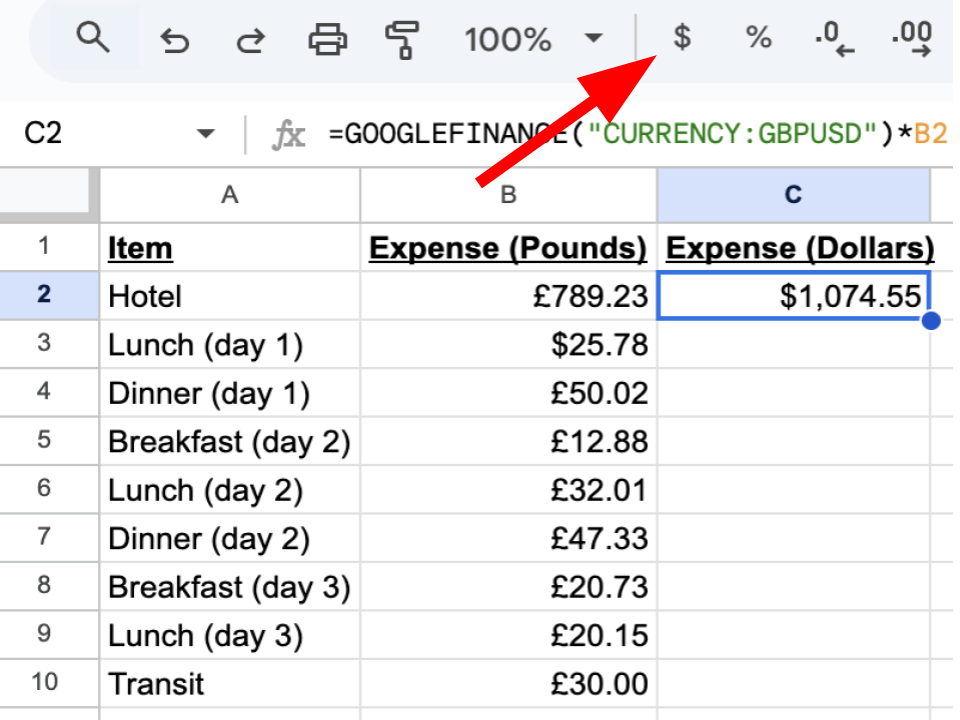
The GOOGLEFINANCE formula will only get you the value of a currency exchange rate, not the formatting. Once you've set up your formula, you'll have to change the formatting manually.

If you're in the US, you'll see a little $ in the menu. Clicking that changes the format of whatever cell you have selected to dollars.

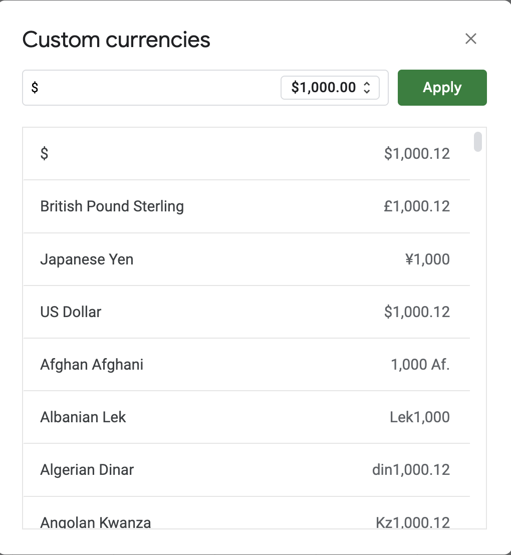
If you don't see that in the menu, or if you want a different currency format, click on Format in the menu, then Number, then Custom Currency.

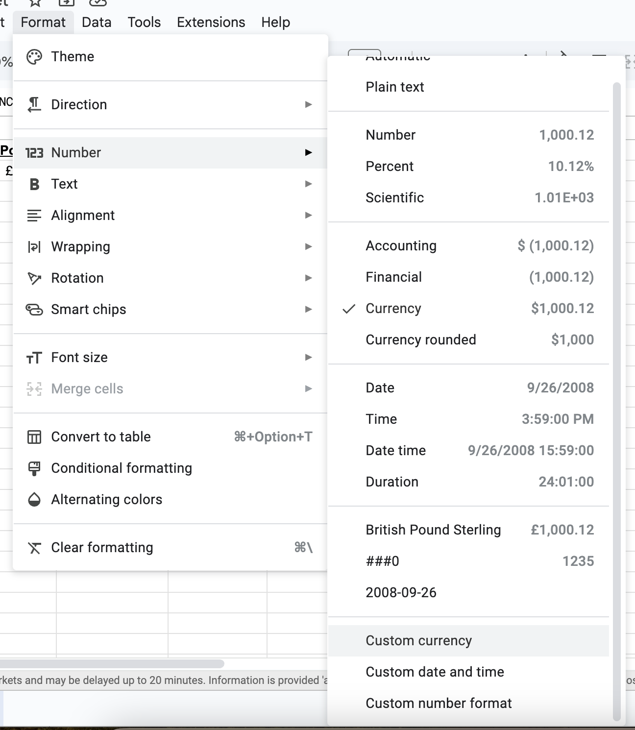
That opens up a menu where you can choose exactly the currency format you want. Just click Apply when you've found it.

(Optional) Step 4: Replace your original values

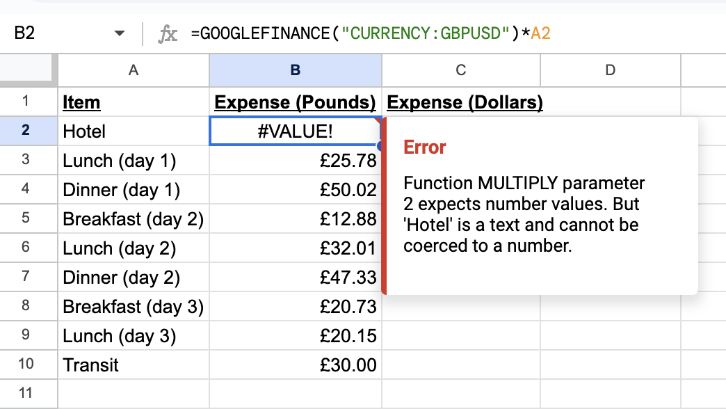
If you don't want to keep your original amounts (in our case, the values in pounds), you can paste the converted values where the original amounts are. But because your formula is based on the first values, just pasting them in will paste the formula, not the value. In our case, that means that the formula in B2 now points to A2, which causes an error.

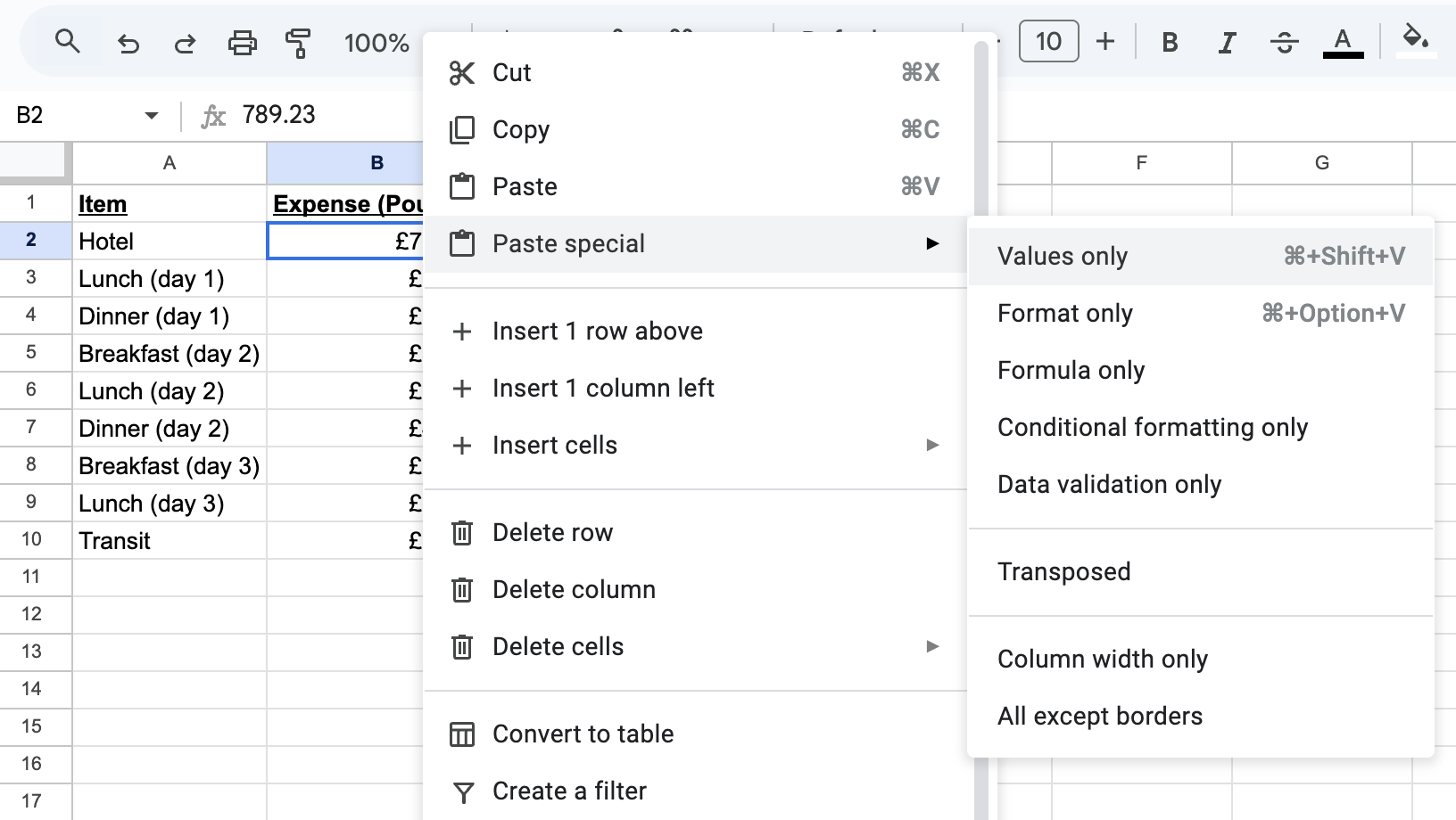
To get around this, you need to paste values. First, copy your converted values (in our case, C2). Next, select the range where you want the converted values. Right click, then choose Paste special, then Values only.

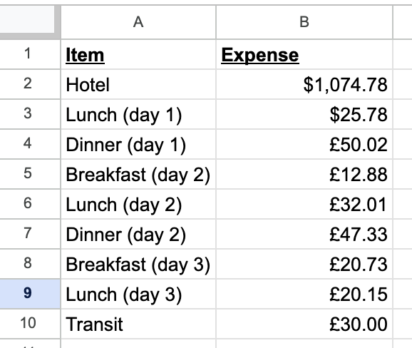
That will replace the original amount with the converted amount. If you haven't fixed the formatting yet, you can do that after pasting. Also be sure to update any labeling on your spreadsheet. In our example, column B was originally labeled Expenses (Pounds), so we've changed it to be less specific.

Step 5: Convert multiple currencies at once

So far we've been converting a single currency pair. But what if you have a column of amounts in different currencies and you want to convert them all to USD?

You can build the formula dynamically using the & operator to join strings. Put your currency codes in a separate column. If column B contains "EUR", "GBP", "JPY", and so on, then in column C, use:

=A2*GOOGLEFINANCE("CURRENCY:USD" & B2)

The & joins "CURRENCY:USD" with whatever is in B2. If B2 contains EUR, Google Sheets reads the formula as GOOGLEFINANCE("CURRENCY:USDEUR"). If B2 contains GBP, it becomes GOOGLEFINANCE("CURRENCY:USDGBP"). Each row looks up its own rate automatically.

Step 6: Apply the formula to many rows

Once you have a formula working in one cell, you don't need to type it again for every row. Select the cell with the formula. You'll see a small blue square at the bottom-right corner. That's the fill handle. Click and drag it down to copy the formula to as many rows as you need.

Google Sheets updates the cell references automatically. If your formula in C2 references A2 and B2, dragging it to C3 gives you a formula that references A3 and B3, and so on.

If part of your formula should stay fixed (for example, if the target currency is in a single cell like D1), use a dollar sign to lock it: $D$1. That tells Sheets not to update that reference when you drag.

Issues with GOOGLEFINANCE for currency

The GOOGLEFINANCE formula works great for most cases, but there are some things you should be aware of.

GOOGLEFINANCE uses the current exchange rate by default

When you use GOOGLEFINANCE("CURRENCY:GBPUSD") without a date, you get today's rate. Tomorrow, the cell will show a different number. For an expense report or invoice you need to lock, that's a problem.

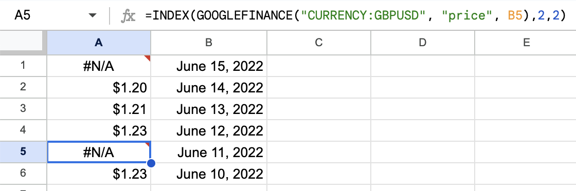
To pin a specific date, you pass a third argument to GOOGLEFINANCE. But there's a catch: adding a date makes GOOGLEFINANCE return a two-row, two-column table (a header row and a data row) instead of a single number. You can't multiply a table by a cell value directly. That's why you need to wrap it in INDEX, which pulls out just the number you want.

The format is:

=INDEX(GOOGLEFINANCE("CURRENCY:[original currency][target currency]", "price", "YYYY-MM-DD"), 2, 2)

The 2, 2 tells INDEX to grab the value in row 2, column 2 of the result. That's where the actual rate sits. To convert £500 at the GBP/USD rate on June 23, 2025:

=INDEX(GOOGLEFINANCE("CURRENCY:GBPUSD", "price", "2025-06-23"), 2, 2) * 500

For a deeper look at date-based lookups, see our guide on historical exchange rates in Google Sheets.

GOOGLEFINANCE errors and how to fix them

#N/A: Google Finance doesn't recognize the currency pair, or the service is temporarily unavailable. First, double-check your three-letter currency code. A typo like GBPUDS instead of GBPUSD will always produce this. If the code looks right, wait a few minutes and try again. Outages usually clear on their own.

#VALUE!: The formula is getting input it doesn't expect. If you're using the dynamic method from Step 5 where you concatenate the currency code from a cell, make sure that cell contains text. If Sheets has interpreted the cell as a number (for example, you typed EUR but it somehow got formatted as a value), the concatenation breaks.

#REF!: A cell that your formula references has been deleted. This usually happens after you delete a row or column. Undo the deletion if you can, or update the formula to point to the correct cell.

GOOGLEFINANCE doesn't update formatting

In our example above, we did manual formatting to get around this. But if you have a lot of conversion to do, it can be a pain to construct the formula, then adjust the formatting.

Instant Currency: An Alternative to GOOGLEFINANCE

Skip the multi-step GOOGLEFINANCE process entirely. Instant Currency converts currencies and formats cells in one click, with reliable historical rates that work even when Google's data fails.

If you have any questions about converting currencies in Google Sheets, drop us a line. We'd love to help you figure it out!